Excel Formula Help - SUMIF for Summarizing Data
In Microsoft Excel, the SUMIF function makes summarizing large data-sets with repetitive entries easier. Thousands of entries over the course of a sales year, for example, can be summarized by individual customer using this function.
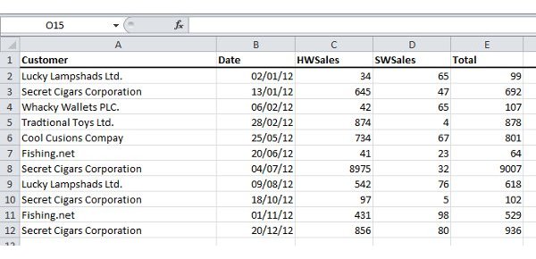
The table below shows an example record of sales specifying separate product areas – hardware and software.
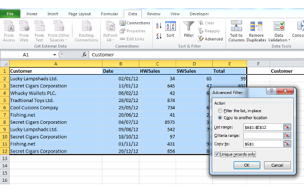
To summarize total sales revenue by customer, first of all we create a new column called Customer and then we select the whole of the original dataset, including headers (there are only 12 entries here but there could be many thousands). Then, from the menu-bar we go to Data and select Advanced from the Sort & Filter section.
We then need to select the Copy to another location radio dial and check the Unique records only function box. Finally, we specify G1 as the output (Copy to) - importantly, note that we are using the '$' symbol to denote absolute references in Excel; This format must be followed:
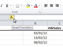
We now have a list of unique customers starting in column G. Your next step is to define the formula in H2 that will extract and total all sales relating to the unique customer in that row. This is done by selecting H2 with the mouse and then choosing the SUMIF formula from the Insert Function fx key:
Click OK and enter the range so that H2 contains the formula =SUMIF($A$2:$A$12,G2,$E$2:$E$12)
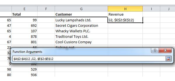
The first unique customer now has the total of their sales from the full data-set in H2. In the formula, both entries for '$12' should be substituted for the number of rows in your data-set. The next step is simply to copy down the formula in H2 for the rest of the unique customers.
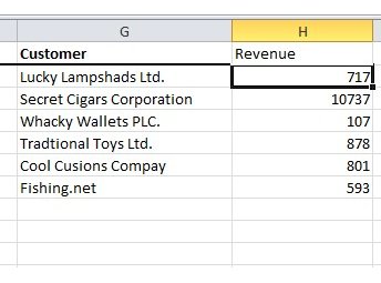
You now have a full summarization of sales revenue by customer. An alternative method for grouping this data would be to use a pivot table, but this formula method shows how sophisticated basic Excel functions can be. For more details on the SUMIF formula, visit the Microsoft Office help page.