Excel Formula Help – VLOOKUP for Changing Percentages to Letter Grades
Following on from an earlier blog, we will now use the VLOOKUP function to convert student percentages to letter grades ranging from F to A+.
First of all, select a couple of columns and write out your grading scale in upside down fashion as shown below. In this format, we are telling VLOOKUP that row 1 says any score above 0 receives an F. The function will then continue filtering down the rows, allocating the relevant letter grades to their respective percentages.
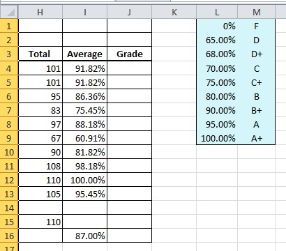
To create the VLOOKUP formula, the easiest way is simply to select the cell, J4, and begin writing =V.. Excel will immediately offer all formulas beginning with the letter V, including VLOOKUP.

Select the function, and start writing your formula. Firstly, you will need the student score argument, I4, followed by the range of your lookup table. Notice in the example below that, like the previous blog, we are again using '$' symbols to create absolute references, this time at each column and row reference in relation to our table coordinates.

We do this so that, as and when we come to copy down, the copy function maintains the lookup table coordinates as a reference whilst changing only the student percentages cell reference. Once copied down, we have our letter grades.

For more on VLOOKUP, check the Microsoft Excel help page. Or, if you would like to build a more complex view of your data using VLOOKUP and other functions, feel free to contact our Excel experts and consultants.