Expert Excel Help – REPT for Quick Data Graphics
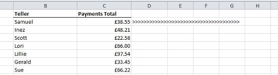
Today's Microsoft Excel help tip is short but sweet. What you will learn is a quick way to represent visual data using the =REPT function. No complex formulas are needed. First of all we have a list of items, in this case a daily tally of cash teller takings in a supermarket.
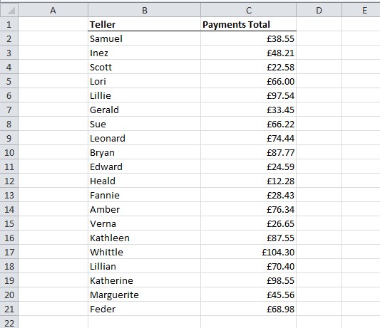
As you can see, takings are listed next to names. What we would like to do is create quick and neat visual representation of these figures without going though the process of creating and formatting a graph or changing the order of the list with a Sort.
First of all, we select the next available cell in the first data row, in this case D2. We then enter the simple formula, =REPT(“>”, C2)
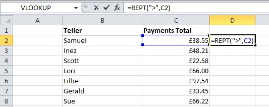
On hitting Return, we see that we get a long line of > symbols. Here, the C2 part of the formula determines the number of symbols to show.
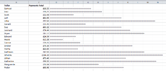
Note that symbols could be anything at all, for example =REPT(“O”, C2) would give us a line of Os.
Next, copy down the formula to to the bottom of the list and your quick and simple visual representation is complete.
For more details of how to use the =REPT formula in Excel, see the Microsoft help pages here.