Excel Formula Help - using RANK to sort entries within a range
The RANK function in Microsoft Excel offers increased control when it comes to sorting numeric values within a range. It also gives us the capacity to include a sorting element to a formula. This blog offers a simple and quick introduction RANK.
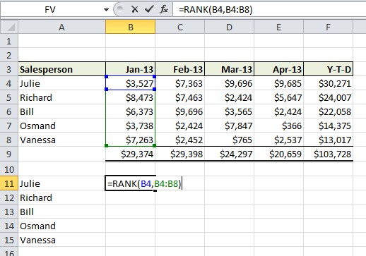
Below we find a sales table which we would like to map into a league-like format showing who was first, second, third etc., i.e. the rank of each sales person, for each month.
We begin by defining the rank of Julie in January. In cell B11, we use the formula format =RANK(number, ref, order) where number=the cell to be ranked, ref=the range of cells with which 'number' will be compared to, and order=whether to rank smallest to largest (ascending) using a 1, or the other way around (descending) using a 0. Use no order switch and the default is descending.
Our formula will be =RANK(B4,B4:B8) No order switch is used as we wish our results to be descending, i.e. the lowest result with be ranked as 5 and the highest as 1.
Before we hit return, we select the cell range and toggle through F4 to assign $ absolute references to both column and row; the range is now fixed and we can copy down.
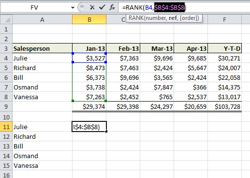
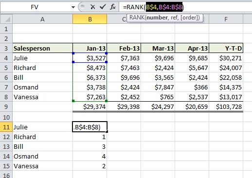
We can edit the formula again, this time using F4 to to apply absolute references so that only rows are anchored, as seen in the formula bar above where the formula now reads =RANK(B$4,B$4:B$8) This allows us to copy across from B11 to F11
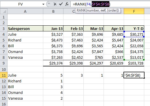
We can now go in and edit each top row formula in row 11 so that when we copy down each row, the rank comparison range is anchored; for example, to rank Y-T-D performaces, we use the formula =RANK(F4,$F$4:$F$8), seen here:
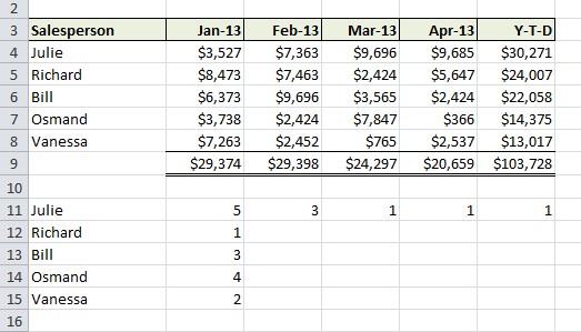
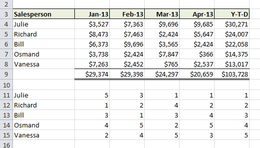
Now, individually copy down each column to create a league table and see rankings for each month, as well as Y-T-D (year to date).
For more help with Excel formulas, contact our experts.