Expert Excel Help - Great Dashboard Visualisations
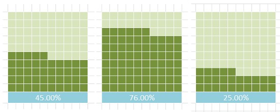
This Microsoft Excel blog offers a quick way to create these dynamic visualizations for your spreadsheets. With these visualisations, each time the percentage at the bottom changes, the number of small colored squares also changes to denote the percentage amount.
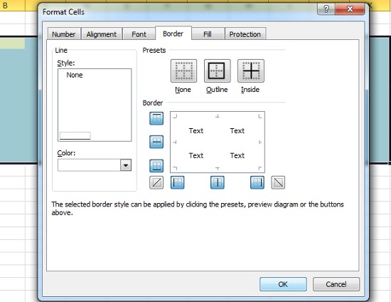
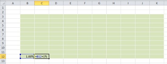
To get here, we begin by selecting 10 x 10 cells and colouring them in any light color. With the cells selected, we use Ctrl 1 as a short cut to bring up the Format Cells options. Here we need to select the Border tab and change the color to white. Under Presents, we also need to select Outline and Inside:
Then, in the bottom left corner, B12, place a value of 1%. Next to that, we create a formula that can be copied across to incrementally increase the value by 1% in each cell, which is: =B12+1%
Select B13 and copy across:

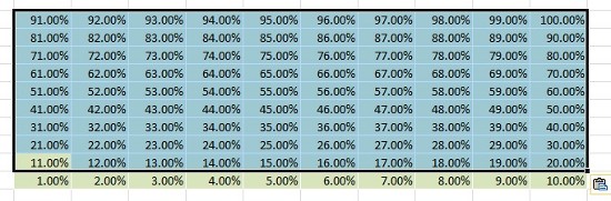
To fill the rest of the table, select B11 and enter the formula, =B12+0.1, like so:

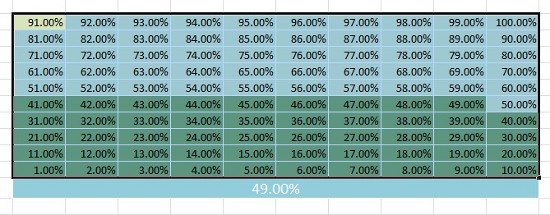
Then copy through the remaining cells. You should now have a table showing 1% to 100%, bottom left to top right, as shown here:
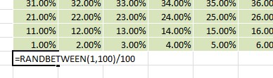
Under the table we then need to create, for the purposes of this demonstration, a random percentage generator. We can do this using RANDBETWEEN, with the formula =RANDBETWEEN(1,100)/100 as shown here:
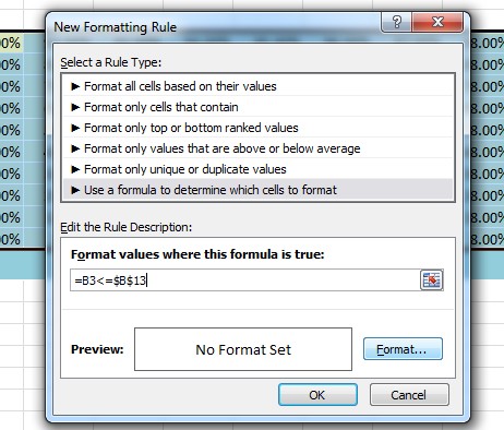
Merge and Centre with colour and increased size. Select the main table and access Conditional Formatting with Ctrl O D (hold down Ctrl and hit O then D). Here select New Rule:
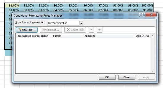
Then the option Use a formula to determine which cells to format. In the Format values where this formula is true space, write the formula =B3<=$B$13 as shown here - then click on Format:
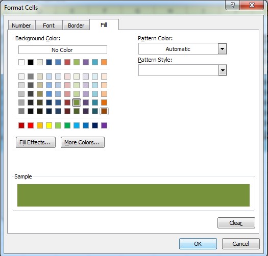
On the Fill tab, select a color that is darker then the main table color, then click OK:
Click OK again,
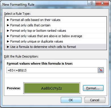
.. and again,
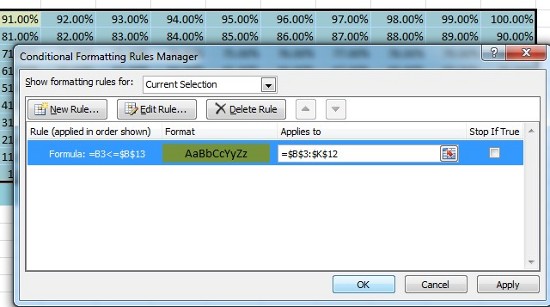
As we can see, the RANDBETWEEN function has generated a value of 49%, in which case, the dark green color is shown up until the 49% cell.
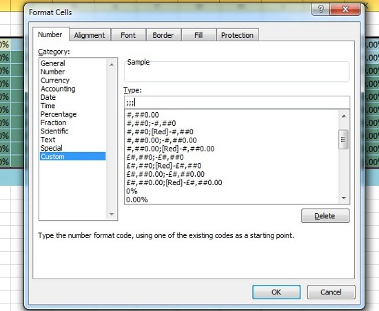
With the main table still selected, we now hit Ctrl 1 again to bring up the Format options again. Select Number and then Custom. In the Type field use three semi-colons ;;; to hide all of the cell values.
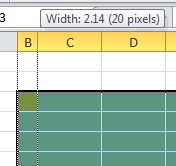
We then need to square off the cells by making the hight and width the same, in this case 20 pixels by 20 pixels. Notice the Excel value for the width is 2.14.
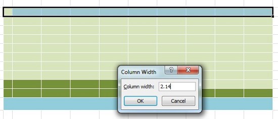
We use this value to scale all the columns by selecting across and using the Column Width short cut Alt O C W (hold down Alt and press O, C, W in order). This brings up the Column Width options box where we type 2.14 and click OK:
Almost done. We can now test our visulziation by repeatedly pressing F9 to cause RANDBETWEEN to auto generate new percentages which are the represented visually:
We can also tidy things up by providing a title and going to the View ribbon to un-check the Gridlines option:
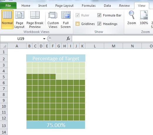
For more Excel tips and advice, contact our experts.