Expert Formula Help - Calculating Employee Health Insurance Costs
The blog gives you a great way of using Microsoft Excel to calculate health insurance costs for employees in your company. The formula will take into account the changing nature of the company headcount by using data from you payroll spreadsheet as a basis for understanding how many employees there are in the company on any given month.
The spreadsheet follows two basic principles. Firstly, that every employee has the same type of insurance at the same cost, $380 per month. Secondly, that insurance is paid immediately on beginning employment with the company. This differers from the common situation where insurance is paid only after a 3 month probationary period with the company.
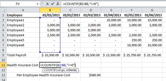
To keep things simple, we will take a six month window beginning from January 2013. As we can see, there have been only two employees that have been with the company throughout the period. Employees 1, 5 and 6 joined the company later on, and employee 3 is no longer on the payroll. All figures represent monthly salaries. Where there are no figures, a 0 (zero) has been used and then by selecting the 0s and using the Comma Style function, (go to the Home ribbon, Number panel and click the large comma), all 0s appear as a hyphen. This makes things look neater whilst at the same time using 0 value which will be required later on.
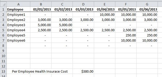
An extra row of 0 values in comma style has been used in case we wish to add further employees.
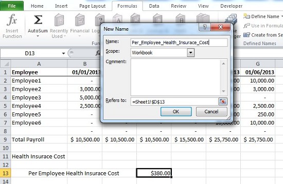
For the sake of clarity, we can total the monthly payroll using a simple SUM function and copied it across:

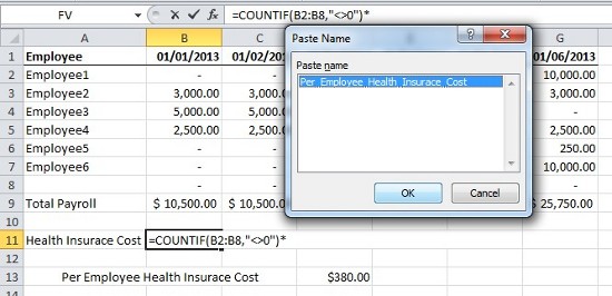
We would then like to take the insurance cost value, here in cell D13, and use the Define Name function to assign it a recognisable text name. First we select the value in D13 and then go to the Formulas ribbon and the Define Names panel. Click on Define Name and an options box appears. Often, any text to the right of the selected cell is automatically used. However, in this case, perhaps because I had merged the cells to the right, nothing was included. In which case, I need to write out the name with no spaces (here I use underscores to fill the spaces).
Click OK and then we can begin looking at our main formula.
The idea here is that our formula will simply count the number of employees on the payroll in any given month. To do this, we need Excel to count any entries in the month column that do not have a value of 0. We begin in cell B11 with the COUNTIF function which literally COUNTs the range of cells, IF a certain criteria is matched, in this case, if the value is not 0.
Our formula is follows the syntax =COUNTIF(B2:B8,"<>0") Here, we can see that we need to use inverted commas " "around the <> operators with 0. This means that, within the range of cells defined, count only those cells that are not equal to zero; <> means 'not equal to..'.
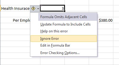
A quick tip: Often when a formula has been written and entered, Excel will notify you of a potential error by leaving a small triangle in the top left corner of the cell. Using the floating drop-down next to the cell, we can see the suggestions Excel has given us to correct or, in our case, ignore the perceived error:
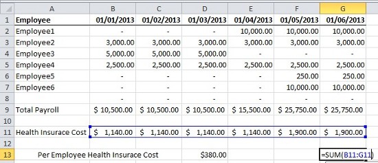
We can now simply return to our formula (hit F2) and multiply the number of employees received from our COUNTIF formula by the insurance value. To do this, add an asterisk * to multiply and then use F3 to bring up the defined name, select it, then click OK:
Our formula should now look like this:
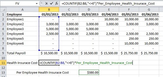
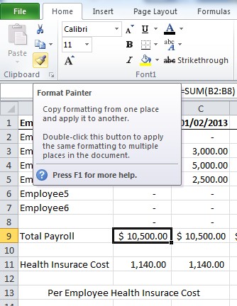
Hit return and we receive the total health insurance costs for each month. The easiest way to get the same formatting as the Payroll totals is to use the format painter (paintbrush symbol) located on the Clipboard pane in the Home ribbon. Fist select the cell which contains the formatted number or text you would like to copy and then click the format painter paintbrush symbol. Now, go to the cell(s) you wish to format and simply select them - they will change their formatting automatically.
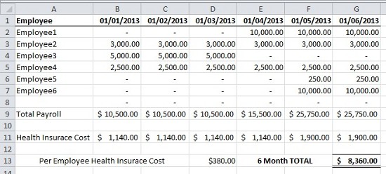
We can go further and get the total insurance cost for the month using a simple SUM of the monthly costs:
And we're done!
For further help with any of your Excel needs, get in touch with our experts. You can also find more help for the COUNTIF function on the Microsoft Excel Help pages here.