Excel Formula Help - Creating an Invoice with dropdowns (Part 1 - Create)
Microsoft Excel is all you need to create a great product specific invoice that will save you time and reduce the possibility of human-error.
Below, we can see a nicely formatted invoice that is so far empty of detail. Below that, (which can be on the same Excel sheet) there is also a separate table which details of stock items, in this case bottles of wine, with prices per unit at wholesale cost. What we would like to do is add a list of items from stock that, when chosen, will have their price auto-filled in the Price column. We would also like to be able to change the Quantity and see the Line Total, and ultimately the Subtotal and Invoice Total calculate correctly.
For this example, I have used a fictitious wine company called Posh Wines.


Firstly, on the left hand side of the invoice, we should select the area where we would like add our product items, which we have done above. We then use the Data Validation tool which can be found under the Data ribbon on the Data Tools pane, as seen here:

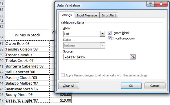
This brings up the options box. On the settings tab under Allow, select List and both the Ignore blank and In-cell dropdown checkbox options. The Data option should greyed out. The Source should be the list of products we would like the dropdown to offer, in this case, our list of wine - select the list and the cell range will automatically be entered with absolute references, as this example shows:
The results are clear when we return to our invoice. Each row now offers a drop down from which any item can be selected.

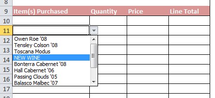
The stock list is also dynamic, so that if we wish to change an item, as can be seen on row 40..

..it will immediately show up in the drop down:
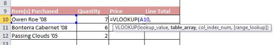
We now have to consider how we are going to get the price of each item to automatically appear in the Price column. For this, we can use a VLOOKUP formula which first of all looks in column A at the entry there for the primary part of the formula, the lookup_value:
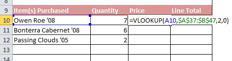
The second part of the formula, as can be seen, is the table_array; for this, we go to our stock table and select the body of the table to provide the formula with data to examine;

Finally, we provide the column number or col _ index _ number where to tell VLOOKUP which results we are looking for (from which column in the table as they are counted from left to right). There is also either a 0 or a 1 at the end of the formula to specify whether we are looking for an exact match to the initial lookup value or a closest match, respectively. We would like an exact match, so we end on 0. The formula should read =VLOOKUP(A10,$A$37:$B$47,2,0)
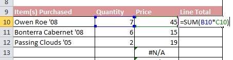
As we have some values in column A already, when we copy the formula down, the prices automatically appear under the Price column. However, we have some ugly error notifications in the cells below as the formula cannot find any values in column A for that row. We will deal with these error signs in a moment.

First, lets complete the table. We have some figures in the quantity column that we would like to use to multiply against our item prices to create a Line Total. This is a fairly straight forward formula, where we can simply use =SUM(B10*C10) or _price multiplied by quantity_, and copy down.
OK, below we can see that we now have two columns with ugly error values; let's get that fixed. First, let's remind ourself of our VLOKKUP formula. As we can see here, VLOOKUP is referencing an empty cell in A13. We need to have a formula that leaves the Price cell empty when there is no data in the corresponding column A cell.

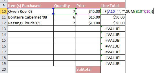
We can do this by adding an IF function to the beginning of the formula and stating that if A10 is empty, enter nothing in the Price cell. This is done with the use of inverted commas or 'speech marks' to denote 'nothing', such as "". So, if "" appears in A10, then enter "" in the Price cell. We amend the formula as shown, not forgetting to add an extra bracket at the end to close off the IF function:
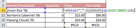
When copied down to replace the present formula, our ugly error values disappear. The same can amendment can be made with the adjacent SUM formula in the Line Total column:
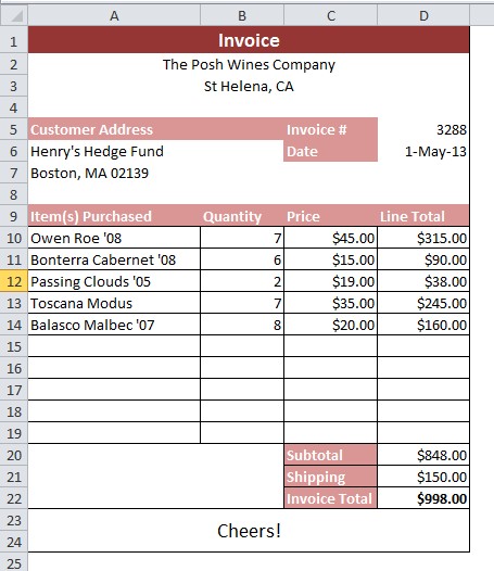
Our semi-automated invoice is almost complete. Now, any bottle of wine from our dynamic stock list can be selected and the price automatically appears. By adding a quantity, the total price is given in the Line Total column:

We then need simply to add the Subtotal with with another SUM formula and include a shipping cost. A further SUM formula to add the Subtotal and to the Shipping will provide us with a fully functioning invoice linked to our stock list.
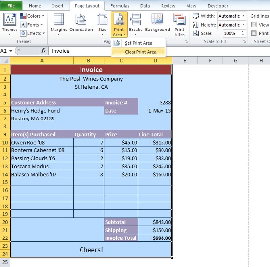
The last thing we need to do is to print a hard copy. The best way to get this done is to select the relevant cells and go to the Page Setup pane on the Page Layout ribbon. First, select Print Area option and click on Clear Print Area. This will reveal what the print area actually is with dotted lines running vertically up and down the sheet:
The next step is to go to the Scale to Fit pane and scale up the print area until it crosses the dotted line:

Once it has crossed, go one step back so that the selected print area fits exactly within the vertical lines:

Follow these instructions carefully and you will be able to print the perfect invoice:

Excel4Business has Excel gurus ready to help you with a vast range of requirements, no matter which industry you are in. For more advice, get in touch.