If asked to draw an Excel spreadsheet, you would probably start by drawing a criss-cross of rows and columns, with letters labelling the columns, and numbers the rows. This layout explicitly shows you the cells and provides a visual cue as to their exact location. When our Excel Programmers develop specialist solutions, we try to leave your sheet looing less utilitarian.
As these features only exist to help you as a user, you do have the ability to hide them. The top image below shows you the standard appearance of your spreadsheet, and the menu from which you can make these changes. Note the View ribbon is selected.
The first image below shows you the effect of unchecking Gridlines (1). You can see the gridlines become hidden. An alternative way of getting the same effect would be to color your entire sheet white though you would not have the ability to toggle between the two views. It is also worth noting that gridlines are, by default, hidden when printing your spreadsheet.
If you hide headings (2), you lose all the letters and numbers marking rows and columns. This has very few disadvantages as you can still see an individual cell's address by selecting it. However, it does remove your ability to easily select, format, insert and delete entire rows and columns. (3) shows you a sheet with the formula and address bar removed. This is generally less useful but, if you are developing a sheet for someone else, it can simplify the interface for them.
The same menu exists in Excel 2007. In earlier versions, all these options can be found under Tools->Options->View. They have been moved because of their popularity.