Our Expert Specialists often freeze panes to ease the visual analysis of data tables within Microsoft Excel. If you use the function correctly, you will always be able to see header rows and columns whilst scrolling through a spreadsheet. However, when you begin to use the function, it may not behave as you expect.
The first step is to work out which rows and columns you wish to view at all times. In (1), we wish to view the names and months. Anything falling under those headings can be considered data. The next step is to select the top left-hand cell within your raw data, in this case Cell A2. When you freeze panes, anything above your selected cell, and to the left of your selected cell, will remain visible at all times. Note this includes hidden cells so make sure you remove any active filters before freezing panes.
Once you have selected the right cell, it is possible to freeze panes simply by selecting that option from the View ribbon (2). Underneath Freeze Panes, you can select to simply freeze the top row or first column. These options do not require you to have selected a cell beforehand. The more general 'Freeze Panes' option will freeze to a specific, selected cell.
After clicking to Freeze Panes, the header rows and columns will display a line underneath and/or to their right (3). As you scroll through your spreadsheet, you can see that the header row (in this case, row 1) is still displayed, even though the first data row displayed is Row 8. Should you wish to reverse the process of freezing panes, you can simply return to the original menu as shown in the image. It may be the case that if you are unable to scroll around your spreadsheet. If so, it could be that a previous user has frozen panes such that all the rows or columns on your screen are technically frozen. Therefore the ability to unfreeze panes can be critical.
In our example, we have looked to display Row 1 and Column A at all times. If we wished to display Rows 1-2, and Column A, we would have selected cell B3 as a starting point. Another common requirement is simply to display the top row. (2) shows there is a shortcut to doing this...but what if you wish to display both Rows 1 and 2? The answer is to select cell A3. As there are no columns to the left, Microsoft Excel will assume you do not wish to freeze any columns. In this case, only a horizontal line gets displayed across the screen.