Expert Excel Help – Tracking Schedules with Conditional Formatting

Here's a great tip for keeping on top of scheduled tasks by using Conditional Formatting in Microsoft Excel 2010, in this case in a for servicing hardware in a mechanical workshop.

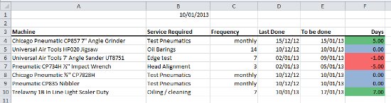
As you can see from the graphic, the final result shows colour coded references to work that is due soon (blue), due today (green) and overdue (red).

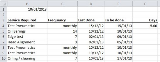
The first thing we need to to do is start with a schedule sheet and add today's date, here in B1. Using the =Today() formula, the present date is added each time we open the spread sheet.

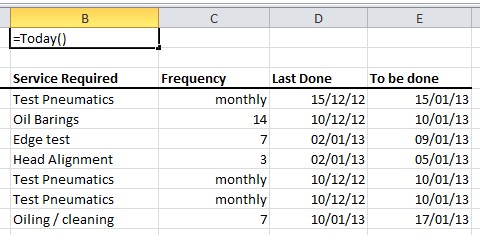
We then add a column called Days in which we need to create a formula that calculates the number of days in relation to today’s date and the To be done date. We do this by entering the formula =E4-$B$1 as seen below (for more on the use of $ symbols, see this earlier blog):

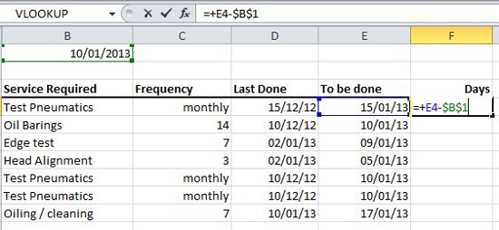
This gives us the correct number of days. In this case we have 5 days until we need to test the equipment again. Once that is done, copy down to cover the rest of the hardware list.

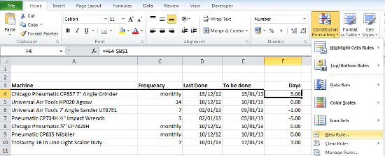
The next thing is to create a colour notification system as seen in the first example above. This is done by using the Conditional Formatting tool. Select it from the Home tab and then click New Rule:

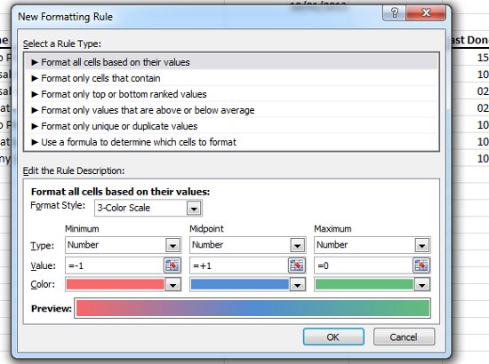
We then get the New Formatting Rule options. Select the first Rule Type to Format cells based on their values and select the 3-color-style from the Format Style drop down, as seen here:

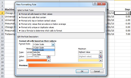
Then simply change to the desired colour scheme and make sure the value Type is Number in each case. The Value field itself should be as follows:

For overdue (red): =-1 For due today (green): =0 For due tomorrow or later (red): =+1

Example:

Again, copy down and your final spreadsheet should now appear as bellow providing you with and easy and quick way to see what tasks need to be completed:

For more on Conditional Formatting, see the Microsoft help pages here or watch this video: