Excel Help - How to Freeze Rows and Columns in Excel 2013
This video will help you learn how to freeze rows and columns in Excel. If you have a large table, but there is valuable information you’d like to see even while you’re working on the rest of the data, you can “freeze” the row so that it is visible at all times.
To freeze the top row or column, Go to the View tab, choose Freeze Panes and click Freeze Top Row or Freeze Top Column.
If you want to select a different row or column that, keep in mind that when you select a cell to freeze panes, the program will freeze the row above or column to the left, so you’ll need to select the row below the row you want to freeze.
Go to the View tab.
Choose Freeze Panes and click Freeze Panes.
Notice the grey line that just appeared – it indicates that the rows above it are frozen and won’t disappear when you start scrolling.
Freezing columns follows the same steps. Note that when you select a column, Excel will freeze the one to its left, so select a column to the right of the one you want to freeze.
Go back to the View tab, choose Freeze panes and click Freeze Panes.
To unfreeze a row or column, go back to the View tab, click Freeze Panes, and click Unfreeze Panes.